
Predictable pricing. Performance improvements. See it for yourself.
Two years ago, we shared our experiences with adopting AWS Graviton3 and our enthusiasm for the future of AWS Graviton and Arm. Once again, we’re privileged to share our experiences as a launch customer of the Amazon EC2 R8g instances powered by AWS Graviton4, the newest generation of AWS Graviton processors. This blog elaborates our Graviton4 preview results including detailed performance data. We’ve since scaled up our Graviton4 tests with no visible impact to our customers.
Our provisional measurements from internal dogfood testing six months ago said that we could “run 25% fewer replicas on the Graviton4-based R8g instances compared to Graviton3-based C7g, M7g, or R7g instances—and additionally 20% improvement in median latency and 10% improvement in 99th percentile latency”—but when it came time to reproduce with a larger sample size in production, we encountered problems where the numbers didn’t look quite like what we saw in our early tests.
Uncovering the mystery
Within our own VPCs, the telemetry path from our production environment through Refinery into dogfood’s Shepherd is very fast. We over-provision Refinery so there should never be a backlog of requests waiting to be sent from production to dogfood—but this is not at all a valid assumption for real-world clients of the production instance of Honeycomb. The effect of network buffering and slow-sending clients becomes noticeable as a fixed cost to latency and throughput. That’s right: Graviton4 is so fast that what previously was a rounding error for receiving off the network and buffering the payload into memory cannot be eliminated no matter how fast the CPU gets.
So we had to rejigger our instrumentation to separately measure network receive time, deserialization time, metrics translation time, and time to serialize and produce payloads into Kafka. In the course of gathering this data, we discovered that our gRPC instrumentation excluded network read and payload decompression/parsing time from the duration of server spans, while our HTTP instrumentation’s server spans included network read and payload decompression/parsing time as part of their duration. We had spans for many of these, but we found it convenient to add attributes onto the root spans for consistency and ease of querying.

Detailed data
Once we cleaned up the data to get separate information for each part of our ingest process, here is what we saw, starting with the network read component:
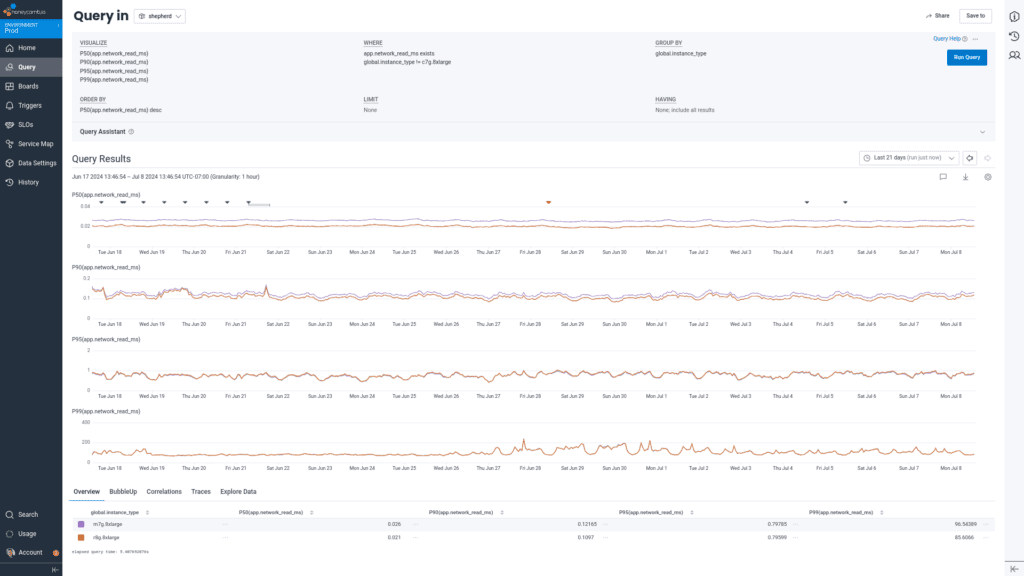
We also saw the p50 network read latency for non-gRPC requests decrease by 6us from 26us to 21us, but p90 network read latency remained essentially unchanged (122us to 110us) and p95+ network read latency was predominated by client behavior (797us at p95, ~80ms at p99). This phenomenon explains why our p99 latency for the overall ingest process was so far off what we observed in dogfood: the p99 network latency began to predominate over processing time.
For gRPC requests, the standard gRPC server interceptor pattern used by our previous beeline instrumentation does not capture time spent reading network bytes off the wire, so we were unable to measure changes to network latency between machine types. We are in the process of upgrading this instrumentation to OpenTelemetry, which supports using the statistics hooks to create spans upon receiving complete request headers, but changes to the instrumentation of our hottest code path were out of scope for this evaluation.
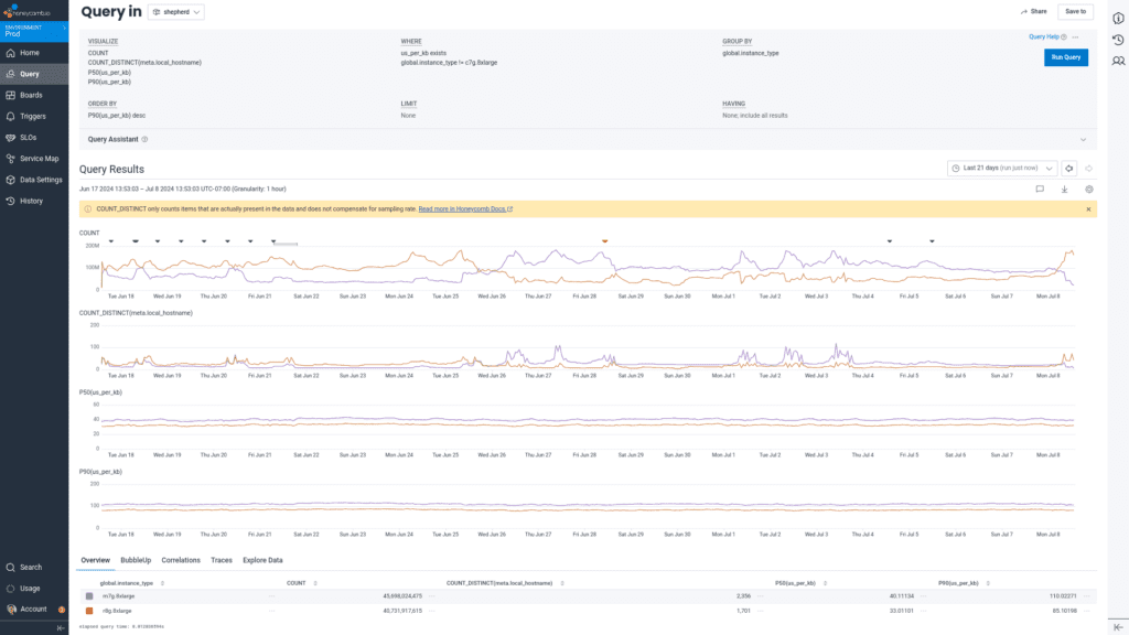
Broadly speaking, processing of any telemetry data inbound into Honeycomb takes five steps: network read, authentication, payload decompression/serialization, reformatting into our internal protocol buffer format (with associated metadata lookups), and writing to Kafka. So having eliminated the network factor, we can move onto the actual real work performed by the CPU.

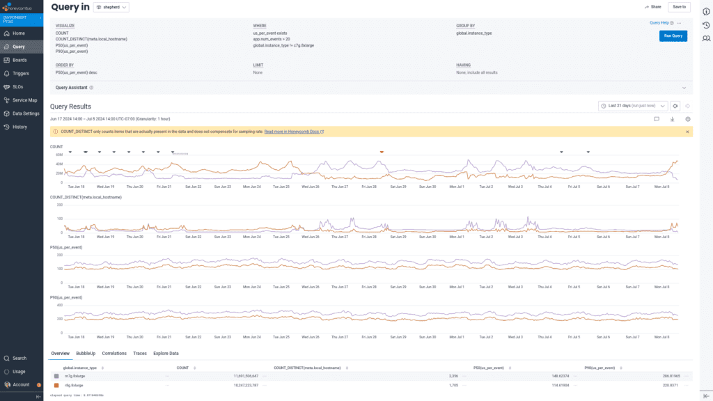
We observed a drop in p50 CPU consumption from 12.8 vCPU per pod to 11.4 vCPU per pod, and p99 CPU consumption from 15.5 vCPU per pod to 14.0 vCPU per pod, while serving 23% more requests per pod.
Breaking out the data by phase of processing after network read, we saw a drop in p50 payload parse time from 40us to 33us per KB, and in p90 payload parse time from 110us to 85us per KB.
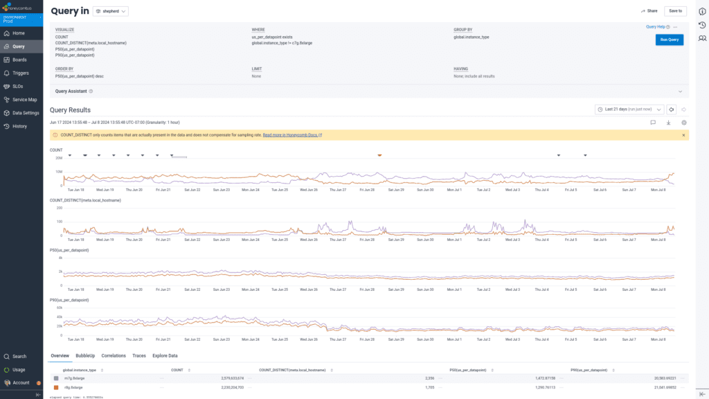
Metrics in Honeycomb are a special case because we expend significant resources reformatting them to ensure events sharing the same target fields are compacted and normalized by time. We saw a drop in p50 metrics to event compaction time from 1.47ms to 1.29ms per flat metric datapoint, and in p99 from 177ms to 158ms per histogram processed (note: metric event compaction is a bimodal distribution; flat metrics compaction is very fast, histogram processing is slower, so the p99 represents the second peak).
Finally, for the stage in which we persist the data to Kafka in our custom protocol buffer format:
We saw a drop in p50 Kafka produce time from 149us to 115us per event, and in p90 Kafka produce time from 287us to 221us per event.
Putting it all together into aggregate time per byte, using 1kb and one event as roughly interchangeable:

Overall, after excluding the network read effects, this resulted in approximately:
- 22% decrease in both p50/p99 processing time for gRPC OTel requests
- 22% decrease in p50/p99 processing time for HTTP OTel requests
- 24% decrease in p50/p99 processing time for HTTP JSON requests
- all with 10% lower CPU utilization and 23% more requests sent per task
Challenges/caveats
As with our experimentation with migrating from Graviton2 to Graviton3, we expect that the performance difference between generations is sufficiently large that we cannot use naive autoscaling across both instance families simultaneously. If we were to do so, the less capable instance type would become overwhelmed with traffic and saturate, or the more capable instance type would be underutilized. Improvements to the ALB load assignment algorithms do partially help to allow least-pending-requests allocation, but we would recommend switching all or nothing rather than running for a prolonged period in a mixed configuration.
The only hiccup we ran into with incompatibility vs. previous versions of Graviton was that Graviton4 drops support for the 32-bit instruction state, and thus binaries compiled for the AArch32 architecture will error with “invalid instruction” messages. We run Metabase, which is a third-party piece of software that was only compiled for armhf, so we had to cordon it onto Graviton3 instances only until we could update our scripts and recompile.
Conclusion
If the transition from x86 to Graviton-based instances was most significant in terms of decreases in tail latency, the generational changes from Graviton2 to Graviton3 to Graviton4 are most pronounced in the throughput improvements. The spread of latency remains very narrow, and the median latency keeps dropping (and thus overall throughput increases). In total, we’ve achieved more than double the throughput per vCPU compared to when we started our Graviton journey four years ago.
The biggest advantage of building on AWS, a cloud provider with a strong track record of silicon innovation, is not having to commit capex to a fixed level of performance for the lifetime of the hardware. Instead, we are able to have confidence each year will give us more bang for our buck as we upgrade our instances while leveraging the same Enterprise Discount Programs (EDPs) and Compute Savings Plans (CSPs).
We are very excited to be able to immediately migrate our entire workload onto Graviton4 as of the general availability of the R8g instance family. And the price-performance improvements allow us to keep innovating and giving you best-in-class observability for the same predictable price. Being able to support distributed tracing across thousands of distinct microservices, and performing whole trace level analytics would not be economical without our infrastructure getting better on its own year on year.
To see these improvements in action, try Honeycomb for free today. To read the announcement from AWS, please head to their blog.


